
The evolution of computer tools has played a key role in the development of the geographic information domain since the end of the 20th century. The joint emergence of information and communication technologies and the increased circulation of data, particularly following the advent of the Internet, have made geomatics a new and indispensable discipline. It uses a specific vocabulary and uses unique technologies called geographic information systems (GIS). GIS use a multidisciplinary and multi-thematic approach for a wide variety of issues in domains such as meteorology, transport networks, marketing, security, agriculture, planning and town planning.
The wide range of definitions describing GIS shows that these systems cannot simply be considered as spatialized data processing software. The definition provided by Françoise de Blomac illustrates this concept well:
“A GIS is an organized combination of computer hardware, software, geographic data and staff capable of entering, storing, updating, manipulating, analyzing and presenting all forms of geographically referenced information” (De Blomac et al., 1994).
Functions of GIS
Several functions can be assigned to these systems, thus making them comprehensive knowledge, decision-making and communication tools.
- The creation and collection of georeferenced data, from multiple sources and highly diverse formats. Examples include the digitization of maps or aerial photographs, the digitization and geocoding of field data, and the spatial, temporal and structural harmonization of data.
- The storage, organization and spatialization of this information via a database management system (DBMS).
- The display and overlay of different layers of geographic information in the form of maps to obtain a spatialized visualization of terrestrial phenomena.
- Querying, spatial and/or statistical analysis to highlight trends and geographic interactions between these different phenomena.
What types of data can be used in a GIS?
Fernandez-Falcon et al. (1993) estimate that over 80% of information has a spatial reference. Technically, these data can be one of two types: images or vectors.
Images, also called rasters, are made up of a matrix of georeferenced pixels to which radiometric color values are assigned. Aerial photographs and topographic maps are examples of commonly used rasters.
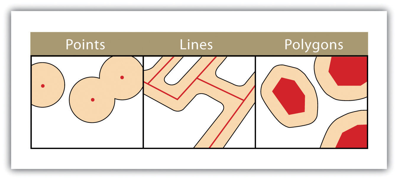
Vector data are composed of geographic objects with basic forms. The points are XY coordinates, the lines are a succession of XY coordinate points and the polygons are a succession of XY coordinate points that delimit a closed surface.
The presentation of all this information in superimposable layers enables users to visualize a real phenomenon.
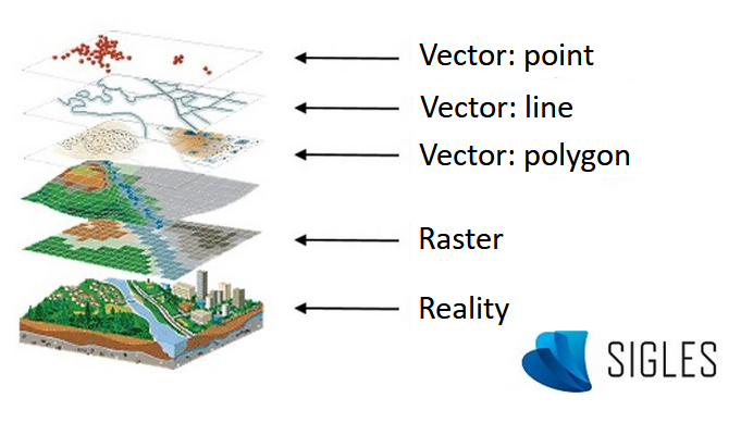
GIS layers (modified, from ESRI France).
Basic spatial analysis tools
GIS provides us with a large number of spatial analysis tools to evaluate the geographic structures and processes of different datasets. These tools are based on different concepts such as distance, spatial interaction and centrality. Powerful spatial analysis tools can be used in the field of environmental health.
Geocoding
Geocoding is used to locate objects or people across the world by transforming a postal address (i.e. an implicit geographic reference) into spatial coordinates (an explicit geographic reference).
⇒ In environmental health, geocoding is used to locate patients via their residential address, or to identify a site sampling point on the map.
Distance / area analysis
This tool is used to identify the closest objects, calculate the area of a polygon, and create buffer zones.
⇒ In environmental health, these tools can be used to generate proximity indicators, including the calculation of how many dangerous industrial sites are located within 10 km of a commune, the identification of patients living within 300 meters of a major road, or the identification of areas that will be affected by a source of pollutants by examining the direction of prevailing winds.
Creation of buffer zones (Campbell J & Shin M, 2011).
Overlay or spatial join
Used to select entities according to the spatial relationship between them and highlight the resulting statistical indicators.
⇒ In environmental health, the spatial join makes it possible to calculate the amount of cultivated land within a given territory and the number and total length of the roads that cross a municipality, or indeed to combine measurements of pollutants carried out within the same geographic area (neighborhood or municipality). These tools can also be used to identify sensitive populations (nurseries, hospitals) that could be exposed to dangers such as industrial hazards or contamination.
Spatial trend analysis
Although mapping is useful when evaluating the spatial trends of a geographic phenomenon, spatial models are needed to understand and quantify these patterns. These models are based on inferential statistics, and assess the significance level of a spatial trend in data: the entities or the values associated with the entities are not a spatially random model in themselves.
⇒ In environmental health, these tools can be used to identify environmental blackspots, i.e. highly polluted and densely populated geographic areas. Although a sampling point with a high pollution value is of interest, it does not necessarily indicate a statistically significant hotspot. A hotspot is indeed considered to exist when an high value is recorded for an entity that is surrounded by other entities that also show high pollution values. In this case, Getis-Ord Gi * spatial statistics software identifies the statistically significant spatial aggregation of high values (hotspots) and low values (coldspots).
Spatial epidemiology tools
The mapping of health data begins with the geocoding of patients via their home address. The data are then aggregated for the most appropriate spatial unit for the study (e.g.: region, county, municipalities or districts).
Disease mapping
Disease incidence mapping is based on the calculation of indicators that have been aggregated within geographic units and shows the proportion of ill individuals within the population: the number of cases of illness per 100,000 inhabitants per commune, for example. These impact indicators are considered to be very “unreliable” for small populations or rare diseases, leading to a result that has high levels of cartographic noise and is difficult to interpret due to the high heterogeneity of population densities within the territory. In addition, showing these indicators as uninterpreted data on a map leads to the individual evaluation of risks in each geographical unit without taking the information provided by neighboring areas into account. Yet the frequency of a disease in a geographic area to those observed in neighboring areas due to the phenomenon of spatial autocorrelation.
“Everything is related to everything else, but near things are more related than far things.” (Waldo Tobler, 1970)
This resemblance phenomenon is used to present reliable maps of the spatial distribution of disease frequency by reducing the variance of the risk estimates through the use of models for smoothing these indicators (Clayton & Kaldor, 1987). These models were developed to provide a more reliable estimation of the spatial structure underlying the incidence and to smooth the background level observed for areas with a low number of cases by sharing the information provided by neighboring units (Elliott & Wartenberg, 2004).
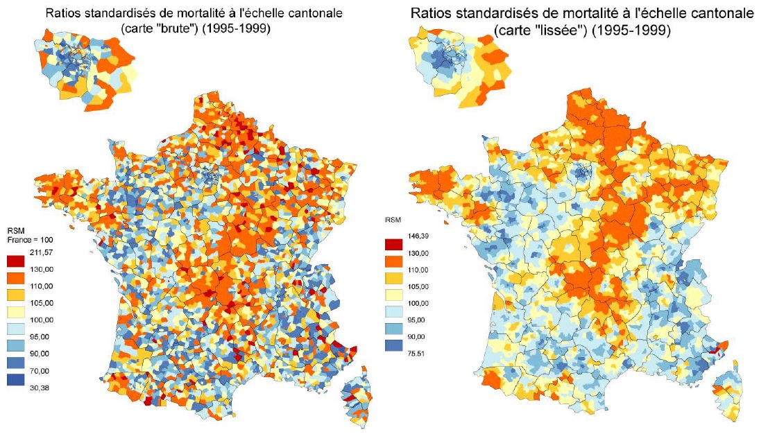
Result of applying smoothing standardized mortality ratios (Rican, 1999).
Several smoothing models are described in the literature (Auchincloss et al., 2012). Those most commonly used to estimate the risks of rare diseases include the hierarchical Bayesian models, and notably that of Besag, York and Mollié (1991), which can simultaneously identify global and local spatial structures.
Cluster detection
Disease mapping techniques are used to assess the spatial heterogeneity of health event incidence. Although these techniques are essential to provide a picture of the geographic distribution, they cannot be used to detect areas of atypical incidence, called clusters, or assess their significance. A cluster is an “abnormally” low or high concentration of cases compared to values that are expected in the area. Spatial scanning methods such as scan statistics can be used to identify these atypical geographic areas.
Developed by Martin Kulldorff in the late 1990s, scan statistics detect clusters of spatial, temporal and spatio-temporal events without any pre-selection bias. This detection can be validated by a significance test for each cluster and can be adjusted according to confounders such as age and sex (Kulldorff 1997; Kulldorff et al. 1998).
This statistics method has two stages. In a first detection phase, the study area is scanned by a window of variable shape and size scans in space and/or time to record the events occurring in the centroid of each geographic unit (geographic center represented by XY coordinates). A probability function (the relative risk: RR) is then calculated for each location and window size according to the distribution of cases of disease and following a Poisson law. The RR depends on the number of cases observed both inside and outside the scan window.
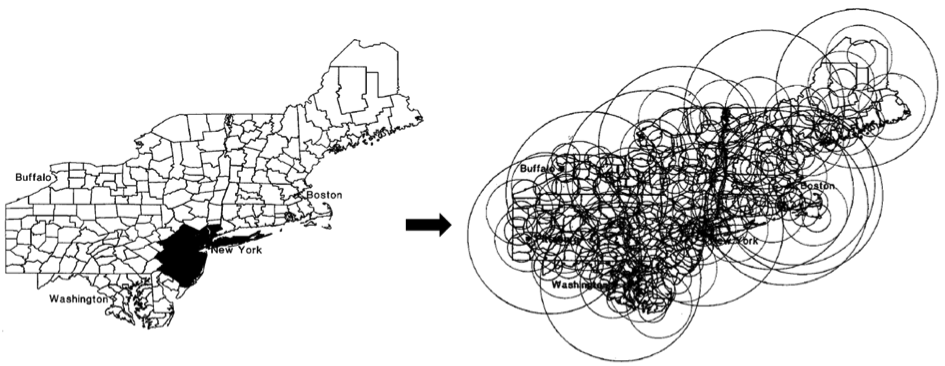
A small sample of the many scan windows used by SaTScanTM (modified from Kulldorff, 1999).
In a second phase, statistical inference is used to determine cluster significance level. The null hypothesis corresponds to the absence of a cluster (the risk is homogeneous and constant across the entire area and/or the study period), and the alternative hypothesis corresponds to the detection of at least one atypical cluster (different levels of risk are observed inside and outside the window).
Scan statistics were first used as an epidemiological application for childhood leukemia and breast cancer mortality in the New York region (Hjalmars et al. 1996; Kulldorff et al. 1997). This method was then widely applied around the world, with more than 200 publications concerning 40 different themes including criminology, botany and archeology listed on the website that offers a free download of the software (SaTScan).
A more advanced version of scan statistics makes it possible to estimate non-homogeneous risks within each cluster detected (Kulldorff, 1999). Indeed, the isotonic version of SaTScanTM can determine several risk levels within the same cluster through a decreasing isotonic regression function according to the distance from the center of the cluster. This function provides additional information, in particular for the precise identification of atypical zones of incidence (epicenter) for large clusters.
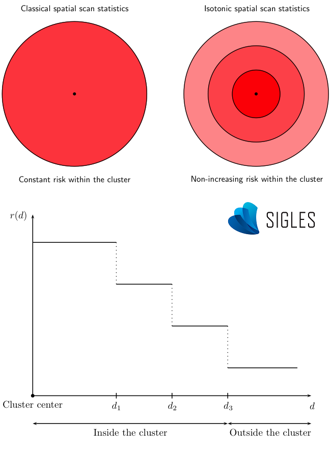
Principle of the isotonic scan statistic.
Spatial interpolation
Most databases from physico-chemical and biological monitoring of the environment can provide geostatistical information. The nature of this information can be defined by quantitative measurements in a sample of spatially geolocated points. The logistics and high costs involved in the collection and analysis of samples requires the prior establishment of sampling plans. The spatial distribution of the samples can then prove to be heterogeneous across the area studied. Through the development of spatial analysis methods, global maps of these indicators of environmental media quality have been created, permitting the assessment of the main trends of each observed phenomenon (Ripley, 1981; Cressie, 1993). Spatial interpolation is a means to carry out the statistical estimation of spatialized data. It is based on the principle that measured and georeferenced point observations provide the most probable value of the observed parameter (called the ‘regionalized variable’) at any geographical point in the spatial domain studied (Hengl, 2007). The result is a cartographic production of estimates for each point of a regular grid that covers the study area.
In environmental health, spatial interpolation can be used to generate pollutant exposure proxies, namely to predict the level of environmental contamination across a geographic area such as a neighborhood or a commune, or even within the specific areas where the patients live.
General principle of spatial interpolation
Different observation points can be used to predict the value of a point for which no sample has been collected by using the simplified mathematical formula of spatial interpolation, which is similar to a weighted arithmetic mean of the observed values (Li & Heap, 2014):
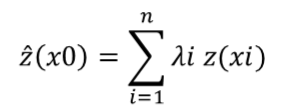
where ^z is the estimated value of the random variable at x0 point of interest, z is the observed value at the sample point xi, λi is the weighting factor assigned to this sample point and n is the number of samples used for estimation.
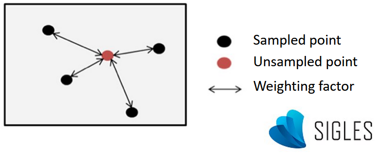
Simplified diagram of spatial interpolation.
Two main approaches
Spatial interpolation methods can be classified according to two main approaches: the deterministic approach and the geostatistical approach. The main difference between these methods is how the weight of each observation point is assigned in the calculation of estimates.
Deterministic methods of interpolation are essentially based on mathematical and geometric properties, and do not consider the spatial structure of the phenomenon. The weighting is linked to the Euclidean distance between the observation site and the prediction site. The closest observation sites therefore have a greater influence in the calculation, while a low or null weight is generally attributed to the most distant sites.
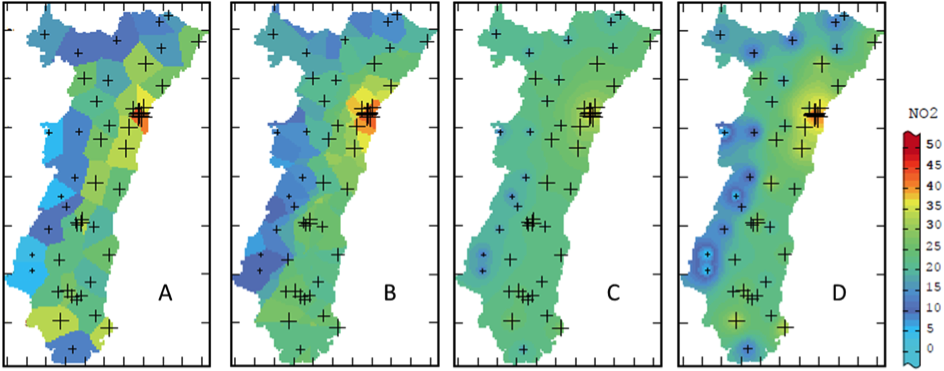
Estimation of the nitrogen dioxide concentration in the Alsace region using different deterministic methods: (A) nearest neighbor, (B) moving average, (C) inverse distance weighting and (D) inverse distance squared weighted interpolation (modified from Lemarchand & Jeannée, 2009).
Probabilistic (or stochastic) interpolation methods are considered to be geostatistical methods because they are directly derived from the geostatistical analysis of observation data and take the concept of natural phenomenon into account (Cressie, 1993; Goovaerts, 1997). As well as using a deterministic structure, these methods include notions of random errors to mimic the spatial behavior of a natural phenomenon (Hengl, 2007). Among these geostatistical methods, kriging is considered to be the optimal interpolation method for environmental phenomena. This method minimizes prediction error by taking the spatial dependence structure of the data into account. Kriging uses observation data and the modeling of an experimental variogram to assign a weight to each of the sites measured using the covariance between these points, according to the distance between them. Here, weighting is a function of several components: the distance between the observed value and the value to be estimated (similar to the deterministic approach), the spatial structure of the sampling (presence of voids or clusters of measured points) and the spatial behavior of the observed phenomenon (fast or slow spatial variability, preferential direction, etc.).
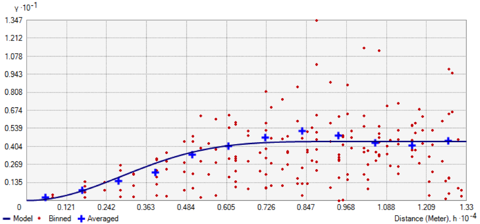
Example of an experimental variogram showing the difference in value between the pairs of points according to the distance between them (ArcGIS® software).
Kriging methods also have other advantages. For example, it is possible to define a more or less significant weight according to the direction (i.e. the anisotropy phenomenon). This makes it possible to consider influences such as the origin of prevailing winds when monitoring a chimney plume, or the direction of river flow when monitoring sediments (Merwade, 2009). Another advantage of certain kriging methods (called co-kriging) is the opportunity to improve the variogram calculation by integrating auxiliary variables that evolve in space in the same way as the regionalized variable (Lemarchand & Jeannée, 2009). However, the most valuable aspect of this method compared to other possibilities is the calculation of a probable estimation error for each unsampled point. This prediction error is generally higher in areas that have few samples and when close to points where extreme values were observed. A phenomenon showing high spatial variability entails higher levels of uncertainty.
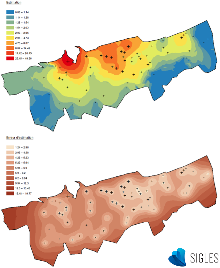
Kriging results (ArcGIS® software). Top: Mapping of the random variable prediction. Bottom: Mapping of prediction error.
References
Auchincloss AH, Gebreab SY, Mair C, Diez Roux AV. 2012. A review of spatial methods in epidemiology, 2000-2010. Annu Rev Public Health, 33: 107-122.
Besag J, York J, Mollié A. 1991. Bayesian image restoration, with two applications in spatial statistics (with Discussion). Annals of the Institute of Statistical Mathematics, 43(1): 1-59.
Campbell J & Shin M. 2011. Essentials to Geographic Information Systems. Flat World Knowledge, Inc. 171p.
Clayton D & Kaldor J. 1987. Empirical Bayes estimates of age-standardized relative risks for use in disease mapping. Biometrics, 43: 671-681.
Cressie NA. 1993. Statistics for Spatial Data (revised edition). John Wiley & Sons, Inc., New York.
De Blomac F, Gal R, Hubert M, Richard D, Tourret C. 1994. Arc/Info, concepts et applications en géomatique. Paris, Hermès, 256 p.
Elliott P & Wartenberg D. 2004. Spatial Epidemiology: Current Approaches and Future Challenges. Environmental Health Perspectives, Vol 112: 998-1006.
Fernandez-Falcon E, Strittholt JR, Alobaida AI, Schmidley RW, Bossler JD, Ramirez JR. 1993. A Review of Digital Geographic Information Standards for the State/Local User. URISA Journal, Vol 5 (2): 21-27.
Goovaerts P. 1997. Geostatistics for Natural Resources Evaluation. Oxford University Press, New York.
Hengl T. 2007. A Practical Guide to Geostatistical Mapping of Environmental Variables. Office for Official Publication of the European Communities, Luxembourg, 143p.
Hjalmars U, Kulldorff M, Gustafsson G, Nagarwalla N. 1996. Childhood leukemia in Sweden: Using GIS and a spatial scan statistic for cluster detection. Statistics in Medicine, 15: 707-715.
Kulldorff M. 1997. A spatial scan statistic. Communications in statistics: theory and methods, 26 (6): 1481–1496.
Kulldorff M, Feuer EJ, Miller BA, Freedman LS. 1997. Breast cancer in northeastern United States: A geographical analysis. American Journal of Epidemiology, 146: 161-170.
Kulldorff M, Athas WF, Feurer EJ, Miller BA, Key CR. 1998. Evaluating cluster alarms: a space-time scan statistic and brain cancer in Los Alamos, New Mexico. Am J Public Health, 88 (9): 1377–1380.
Kulldorff M. 1999. An isotonic spatial scan statistic for geographical disease surveillance. Journal of the National Institute of Public Health, 48: 94–101.
Lemarchand O, Jeannée N. 2009. Méthodes de cartographie et approche géostatistique – La cartographie de la pollution au dioxyde d’azote en Alsace. Cahier des thèmes transversaux ArScAn, 9: 203-214.
Li J & Heap AD. 2014. Spatial interpolation methods applied in the environmental sciences: a review. Environmental Modelling & Software, 53: 173-189.
Merwade V. 2009. Effect of spatial trends on interpolation of river bathymetry. Journal of Hydrology, 371: 169–181.
Rican S. 2007. Représentation cartographique des données sanitaires. Séminaire ORS Île de France « De la mesure des expositions à l’évaluation des conséquences pour la santé : le traitement spatialisé des données ». Paris, 7 septembre 2007. Communication orale.
Ripley BD. 1981. Spatial Statistics. New York: Wiley.
Tobler W. 1970. A Computer Movie Simulating Urban Growth in the Detroit Region. Economic Geography, 46: 234–40.